Formatting the results on the dashboard
You can apply basic and conditional formatting in Excel on the results that you got from running your 1010data query.
Basic Formatting
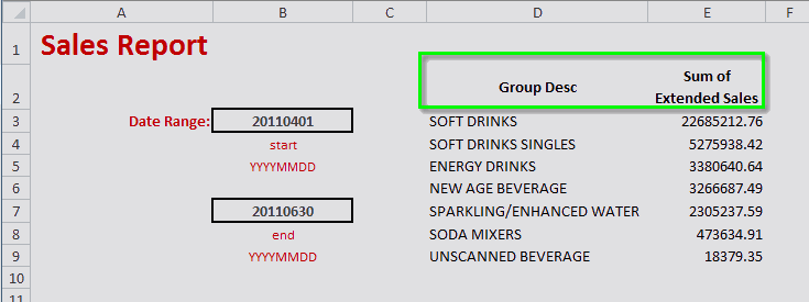
Since this is a dashboard, we can add a little formatting to make it more visually appealing. So, for our query results, let's change the cells containing the column headers to be bold, and let's center the text in those cells both horizontally and vertically.

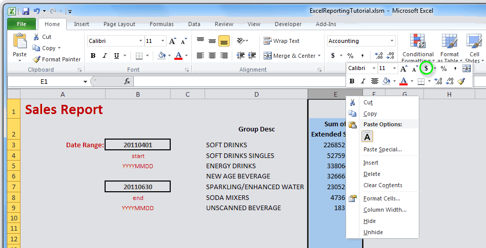
We'll also change the format of the Sum of Extended Sales column to appear as dollar amounts. Right-click the column heading in Excel and click the $ from the context menu:

The values in that column will now be formatted correctly:

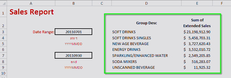
These formats will be retained every time the query is run. We can verify that by changing the dates and running the query again. Change the start date to 20110701 (07/01/2011) and the end date to 20110930 (09/30/2011). To run the query press Ctrl+Q (or click ). When the query finishes running, you should see the following results:

You can see that the values in the Sum of Extended Sales column have changed to reflect the new date range, and the formatting has been kept intact.
Conditional Formatting
We can also incorporate conditional formatting for the results from our 1010data query within our Excel workbook. Let's say we want the format the range of values in the Sum of Extended Sales column using a color scale. On the Home tab, click the Conditional Formatting button, and select Manage Rules... from the menu. The Conditional Formatting Rules Manager dialog is presented:

Let's create a rule to apply conditional formatting using a color scale:
- Click the New Rule... button.
- In the New Formatting Rule dialog, change the Format Style to 3-Color Scale, then click OK.
- In the Applies to field, enter =query_results_range, so that the rule will be applied to any of the values that appear within the range we defined for our results earlier.
- Click Apply to create the new rule.
- Click the New Rule... button.
- From the Select a Rule Type list, select Format only cells that contain.
- Under Edit the Rule Description, make sure the first drop-down is Cell Value, change the second drop-down to less than, and enter 0 in the third drop-down.
- Click the Format button.
- In the Format Cells dialog, click the Fill tab.
- Under Background Color, click the red box, then click OK.
- In the New Formatting Rule dialog, click OK .
- In the Conditional Formatting Rules Manager dialog, in the Applies to field, enter =query_results_range.
- Click OK .
The results of our query are now formatted with a color scale:

Our dashboard now shows us the total sales in a certain department within a specified date range and groups those results by the values in the Group Desc column in the Product Master table. These results are also conditionally formatted using a color scale.
Let's add a simple chart to the dashboard to visually represent these results.
