Weighted Least Squares Regression

In this example, a weighted least squares regression is applied to a data set containing weighted census data to show the relationship between both the age and education level of a worker and that person's income.

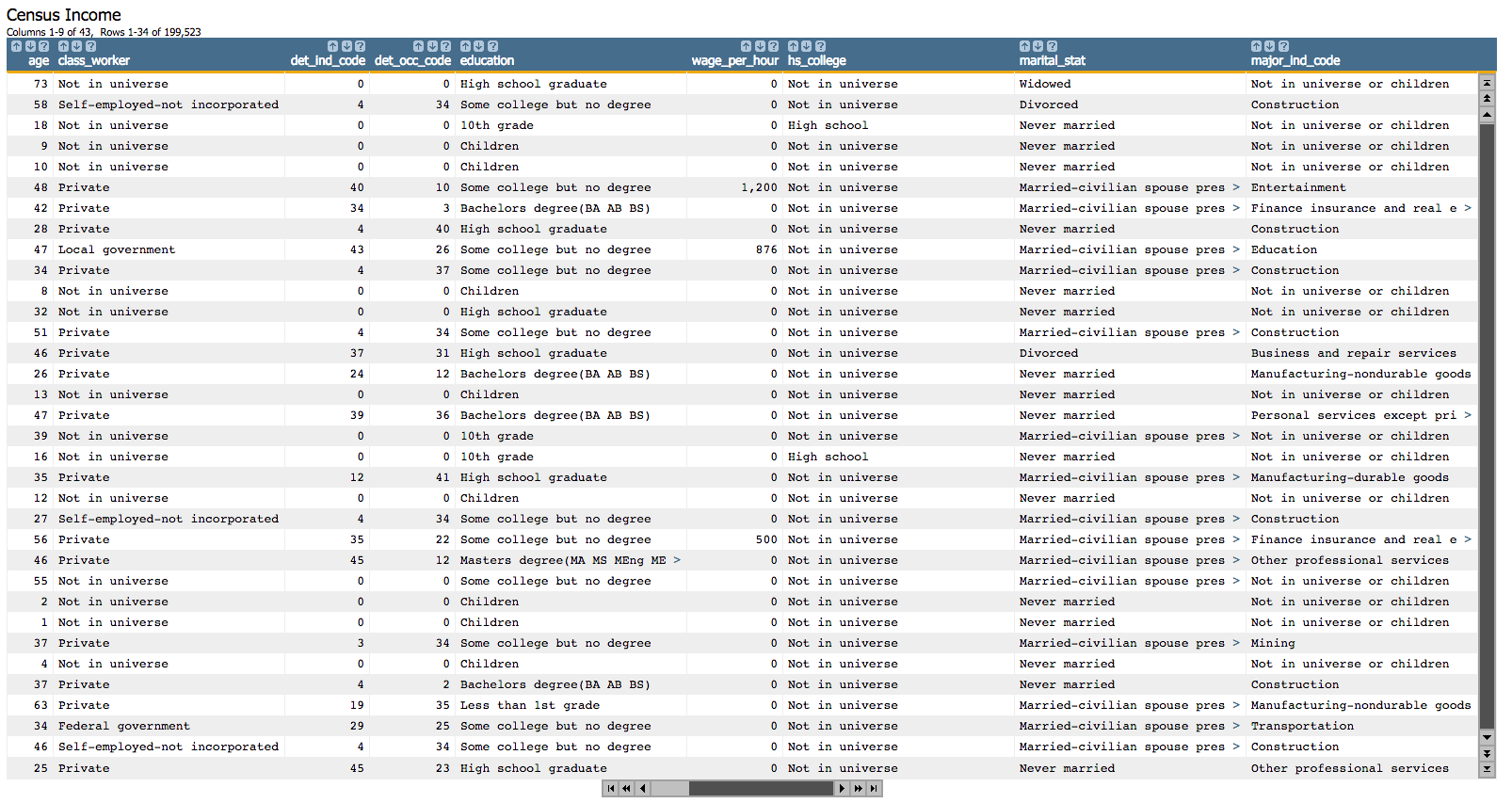
1. Open the Census Income data set (pub.demo.mleg.uci.censusincome).

   

2. Select only those rows where wage_per_hour is not equal to 0, since we only want to do the regression for those people who have a job.

   <sel value="(wage_per_hour<>0)"/>

3. Since we're using age as a predictor, let's see if it has a linear relationship to wage_per_hour, our response.
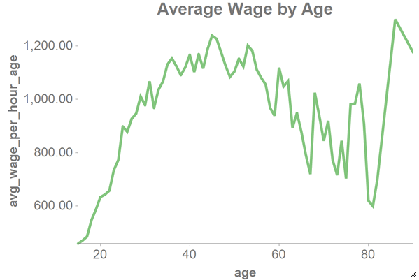
   1. For visualization purposes, we can look at the relationship between the average wage per hour and age.

      Let's first calculate the average wage per hour grouping by age. We'll use the function g_avg(G;S;X) and we'll specify the age column for the G parameter (we're grouping by age) and wage_per_hour as the X parameter (since we want to calculate the average wage per hour). We'll omit the S parameter since we want to consider all rows in the table.

      <willbe name="avg_wage_per_hour_age" value="g_avg(age;;wage_per_hour)" 
      format="dec:2"/>

   2. Click Chart > Line.
   3. Drag the age column to the DATA (X-AXIS) area.
   4. Drag the avg_wage_per_hour_age column to the DATA (Y-AXIS) area.
   5. Click Update.

      

      Since we can see from this chart that the relationship between age and wage_per_hour has a quadratic form, we will include the square of the age as one of the predictors.

4. Let's create a column containing the square of the value in the age column, which we will use as one of the predictors.

   <willbe name="age_sq" value="age^2"/>

5. Since we're also using edu_year as a predictor, let's see if it has a linear relationship to wage_per_hour.
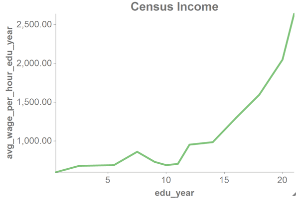
   1. For visualization purposes, we can look at the relationship between the average wage per hour and years of education.

      Let's first calculate the average wage per hour grouping by years of education. We'll use the function g_avg(G;S;X) and we'll specify the edu_year column for the G parameter (we're grouping by years of education) and wage_per_hour as the X parameter (since we want to calculate the average wage per hour). We'll omit the S parameter since we want to consider all rows in the table.

      <willbe name="avg_wage_per_hour_edu_year" value="g_avg(edu_year;;wage_per_hour)" format="dec:2"/>

   2. Click Chart > Line.
   3. Drag the edu_year column to the DATA (X-AXIS) area.
   4. Drag the avg_wage_per_hour_edu_year column to the DATA (Y-AXIS) area.
   5. Click Update.

      

      We can see from this chart that the relationship between edu_year and wage_per_hour has a linear form.

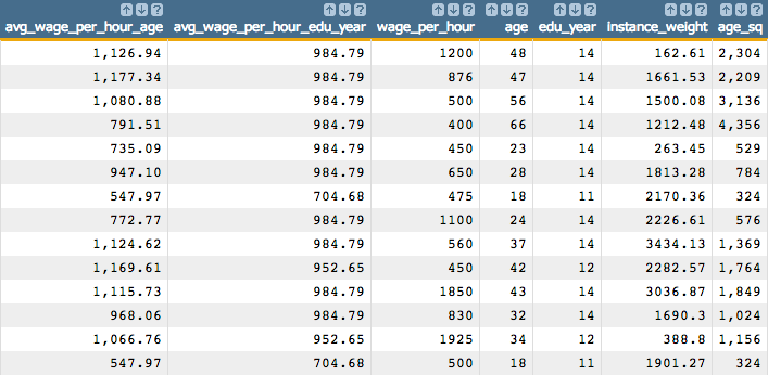
6. Now, let's show only those columns that we are going to use in the model (as well as those we used in the charts from the previous steps).

   <colord cols="avg_wage_per_hour_age,avg_wage_per_hour_edu_year,
   wage_per_hour,age,edu_year,instance_weight,age_sq"/>

   

7. Next, we fit our model on the three predictors as well as the response that we have selected using the g_wlsq(G;S;Y;W;XX) function.

   <willbe name="model_wlsq" value="g_wlsq(;;wage_per_hour;instance_weight;1 age age_sq edu_year)"/>

   Note: As the first element of XX, we specify the special value 1 for the constant (intercept) term in the linear model.

   This creates a column named model_lsq that contains the results of the least squares regression:

   

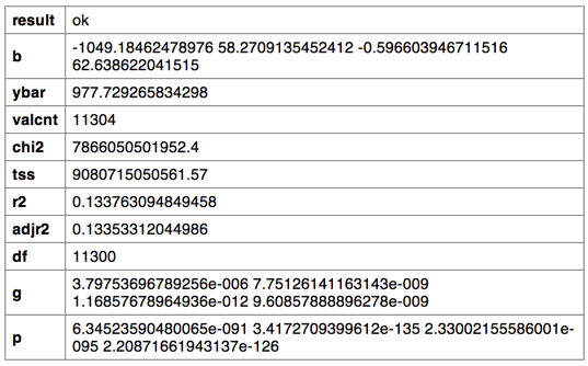
   Clicking on the > opens a window containing a summary of the model output:

   

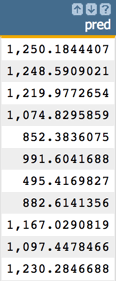
8. We can then obtain the predicted value of the linear model using the score(XX;M;Z) function.

   <note>OBTAIN MODEL SCORE WITH SCORE FUNCTION</note>
   <willbe name="pred" value="score(1 age age_sq edu_year;model_wlsq;)" format="dec:7"/>

   Note: We specify format="dec:7" so that our results show with 7 decimal places.

   

9. To obtain the coefficients of the linear model, we can use the param(M;P;I) function.

   In the following Macro Language code, we obtain the parameters for the intercept (b0) and the first two variables (b1 and b2).

   <note>OBTAIN MODEL COEFFICIENTS</note>
   <willbe name="b0" value="param(model_wlsq;'b';1)" format="dec:7"/>
   <willbe name="b1"value="param(model_wlsq;'b';2)" format="dec:7"/>
   <willbe name="b2" value="param(model_wlsq;'b';3)" format="dec:7"/>

   

10. We can also obtain the p-values of the coefficients using the param(M;P;I) function. We will use these to conduct the variable selection later in the analysis.

    In the following Macro Language code, we obtain the p-value for the intercept (p0) and the first two variables (p1 and p2).

    <note>OBTAIN P-VALUES</note>
    <willbe name="p0" value="param(model_wlsq;'p';1)"/>
    <willbe name="p1" value="param(model_wlsq;'p';2)"/>
    <willbe name="p2" value="param(model_wlsq;'p';3)"/>

    

11. However, one might want to obtain all of the coefficients in one column and the p-values in another, which can be achieved with the following Macro Language code:

    <note>CALCULATE ALL COEFFICIENTS IN ONE COLUMN AND P-VALUES IN ANOTHER</note>
    <willbe name="var_names_1" value="'intercept,age,age_sq,edu_year'"/>
    <willbe name="temp_i_1" value="mod(i_(1);4)"/>
    <willbe name="i_1" value="if(temp_i_1=0;4;temp_i_1)"/>
    <willbe name="b_1" value="param(model_wlsq;'b';i_1)" format="dec:7"/>
    <willbe name="p_1" value="param(model_wlsq;'p';i_1)"/>
    <willbe name="var_name_1" value="csl_pick(var_names_1;i_1)"/>

    

    Note: The number of coefficients and p-values we obtain from the linear model corresponds to the number of variables in our analysis. So, for our example, we obtain 4 coefficients and 4 p-values, which correspond to the intercept plus the 3 predictors.
12. Using the param(M;P;I) function, we can obtain various statistics for this model such as the degrees of freedom of the model, residual sum of squares, mean squared error, number of observations, average of Y, R², and adjusted R².

    <note>OBTAIN VARIOUS MODEL STATISTICS</note>
    <willbe name="dof" value="param(model_wlsq;'df';)"/>
    <willbe name="sse_temp" value="(wage_per_hour-pred)^2"/>
    <willbe name="sum_sq_resids" value="g_sum(;;sse_temp)" format="dec:7"/>
    <willbe name="mean_sq_err" value="sum_sq_resids/dof" format="dec:7"/>
    <willbe name="num_observations" value="param(model_wlsq;'valcnt';)"/>
    <willbe name="avg_y" value="param(model_wlsq;'ybar';)" format="dec:7"/>
    <willbe name="R_squared" value="param(model_wlsq;'r2';)" format="dec:7"/>
    <willbe name="adjusted_R_squared" value="param(model_wlsq;'adjr2';)" format="dec:7"/>

    

    

13. We can calculate the AIC using the following Macro Language code:

    <note>CALCULATE AIC</note>
    <willbe name="sum_log_likelihood" value="loge(sum_sq_resids/num_observations)"/>
    <willbe name="num_of_var" value="3"/>
    <willbe name="AIC" value="2*num_of_var+num_observations*sum_log_likelihood"/>

    

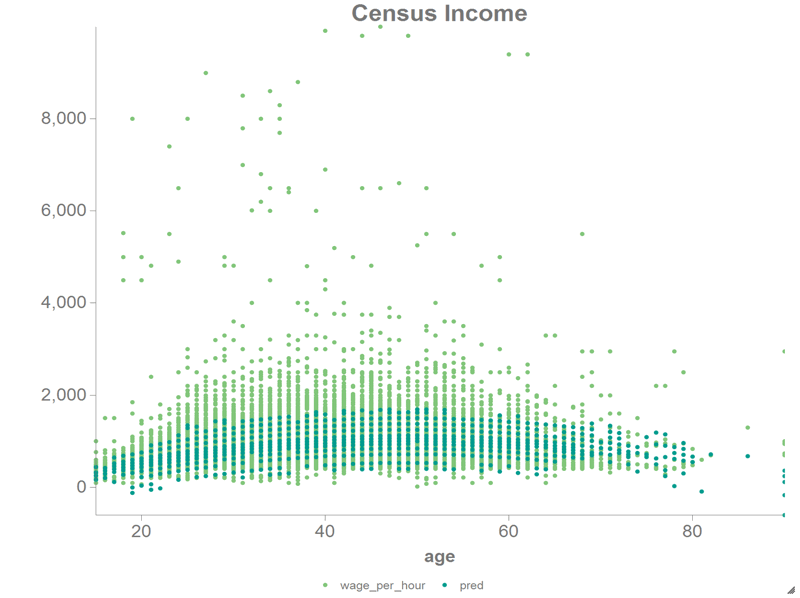
14. Finally, we can visualize the results of the weighted least squares regression using the 1010data Chart Builder.
    1. Click Chart > Scatter.
    2. Drag the age column to the DATA (X-AXIS) area.
    3. Drag the wage_per_hour and pred columns to the DATA (Y-AXIS) area.
    4. Click Update.

    The results should look similar to the following chart: