Least Squares Regression

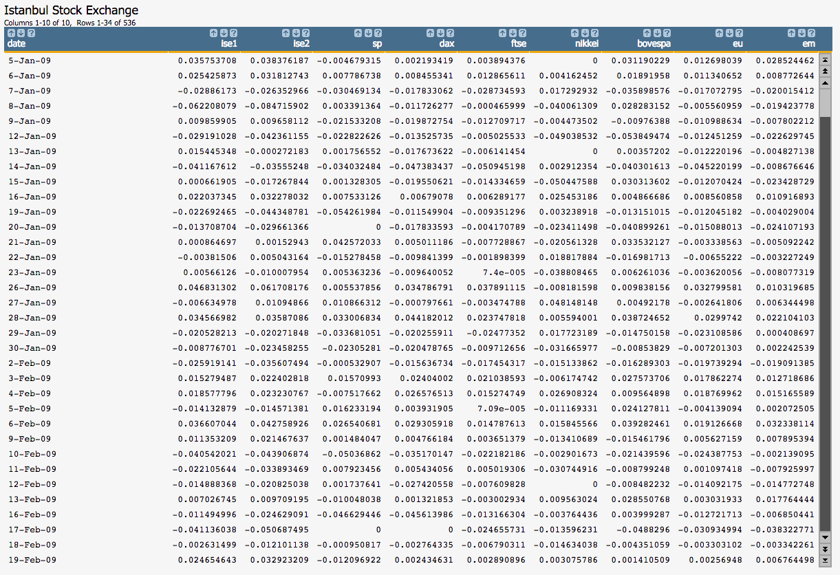
In this example, a least squares regression is performed on a data set containing the returns of a number of international stock exchanges and is used to show the linear relationship between the Istanbul Stock Exchange and the other exchanges.

1. Open the Istanbul Stock Exchange data set (pub.demo.mleg.uci.istanbul).

   

2. Run the model on the seven predictors as well as the response that we have selected using the g_lsq(G;S;Y;XX) function.

   <willbe name="model_1" value="g_lsq(;;ise2;1 sp dax ftse nikkei bovespa eu em)"/>

   Note: As the first element of XX, we specify the special value 1 for the constant (intercept) term in the linear model.

   This creates a column named model_1 that contains the results of the least squares regression:

   

   Clicking on the > opens a window containing a summary of the model output: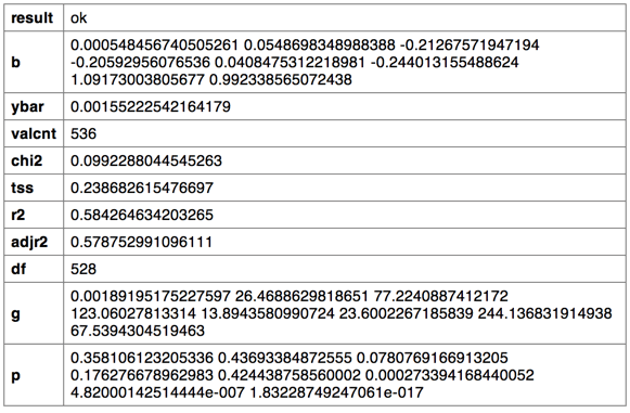

   

3. We can then obtain the predicted value of the linear model using the score(XX;M;Z) function.

   <note>OBTAIN MODEL SCORE WITH SCORE FUNCTION</note>
   <willbe name="pred_1" value="score(1 sp dax ftse nikkei bovespa eu em;model_1;)" format="dec:7"/>

   Note: We specify format="dec:7" so that our results show with 7 decimal places.

   

4. To obtain the coefficients of the linear model, we can use the param(M;P;I) function.

   In the following Macro Language code, we obtain the parameters for the intercept (b0) and the first two variables (b1 and b2).

   <note>OBTAIN MODEL COEFFICIENTS</note>
   <willbe name="b0" value="param(model_1;'b';1)" format="dec:7"/>
   <willbe name="b1" value="param(model_1;'b';2)" format="dec:7"/>
   <willbe name="b2" value="param(model_1;'b';3)" format="dec:7"/>

   

5. We can also obtain the p-values of the coefficients using the param(M;P;I) function. We will use these to conduct the variable selection later in the analysis.

   In the following Macro Language code, we obtain the p-value for the intercept (p0) and the first two variables (p1 and p2).

   <note>OBTAIN P-VALUES</note>
   <willbe name="p0" value="param(model_1;'p';1)" format="dec:7"/>
   <willbe name="p1" value="param(model_1;'p';2)" format="dec:7"/>
   <willbe name="p2" value="param(model_1;'p';3)" format="dec:7"/>

   

6. However, one might want to obtain all of the coefficients in one column and the p-values in another, which can be achieved with the following Macro Language code:

   <note>CALCULATE ALL COEFFICIENTS IN ONE COLUMN AND P-VALUES IN ANOTHER</note>
   <willbe name="var_names_1" value="'intercept,sp,dax,ftse,nikkei,bovespa,eu,em'"/>
   <willbe name="temp_i_1" value="mod(i_(1);8)"/>
   <willbe name="i_1" value="if(temp_i_1=0;8;temp_i_1)"/>
   <willbe name="b_1" value="param(model_1;'b';i_1)" format="dec:7"/>
   <willbe name="p_1" value="param(model_1;'p';i_1)" format="dec:7"/>
   <willbe name="var_name_1" value="csl_pick(var_names_1;i_1)"/>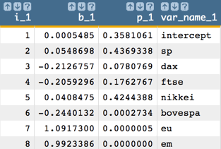

   

   Note: The number of coefficients and p-values we obtain from the linear model corresponds to the number of variables in our analysis. So, for our example, we obtain 8 coefficients and 8 p-values, which correspond to the intercept plus the 7 predictors.
7. We now perform a stepwise regression using backward elimination.

   We start by eliminating the variable that has the largest p-value greater than 0.05. Then, we run the model with the remaining variables. We repeat this process until all the remaining predictors' p-values are less than 0.05.

   1. In our example, sp has the largest p-value that is greater than 0.05, so we want to eliminate that variable and run the model with the remaining 6 variables.

      <willbe name="model_2" value="g_lsq(;;ise2;1 dax ftse nikkei bovespa eu em)"/>

   2. Next, we obtain the predicted value for this second model.

      <willbe name="pred_2" value="score(1 dax ftse nikkei bovespa eu em;model_2;)" format="dec:7"/>

   3. Then, we obtain all of the coefficients and p-values.

      <willbe name="var_names_2" value="'intercept,dax,ftse,nikkei,bovespa,eu,em'"/>
      <willbe name="temp_i_2" value="mod(i_(1);7)"/>
      <willbe name="i_2" value="if(temp_i_2=0;7;temp_i_2)"/>
      <willbe name="b_2" value="param(model_2;'b';i_2)" format="dec:7"/>
      <willbe name="p_2" value="param(model_2;'p';i_2)" format="dec:7"/>
      <willbe name="var_name_2" value="csl_pick(var_names_2;i_2)"/>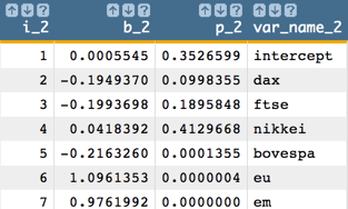

      

      Note: Once again, the number of coefficients and p-values we obtain from the linear model corresponds to the number of variables in our analysis. So, for our example, we obtain 7 coefficients and 7 p-values, which correspond to the intercept plus the 6 predictors.
   4. Now we eliminate the next variable which has the largest p-value greater than 0.05 (which, in our example, is nikkei).

      Then run the model with the remaining variables, which results in the following:

      

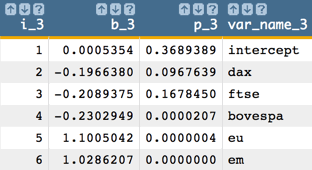
   5. The next variable to drop is the intercept. Then we run the model with the remaining variables.

      

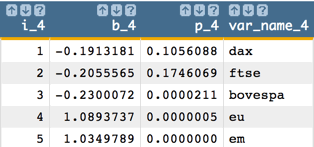
   6. Next, drop ftse and run the model again: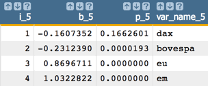

      

   7. Now, drop dax and run the model again: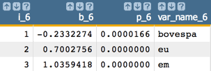

      

   Finally, all of the remaining predictors' p-values are less than 0.05.

   So, the final model is:

   Y = -0233*bovespa + 0.700*eu + 1.036*em

   In our example, the final model is in the column named model_6 and the final predicted value is pred_6.

   For clarity in the calculations going forward, let's put our results in the more generically named columns: model and pred.

   <willbe name="model" value="model_6"/>
   <willbe name="pred" value="pred_6"/>

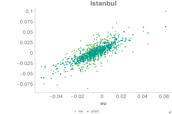
8. We can visualize the results of the least squares regression using the 1010data Chart Builder.
   1. Click Chart > Scatter.
   2. Drag the eu column to the DATA (X-AXIS) area.
   3. Drag the ise and pred columns to the DATA (Y-AXIS) area.
   4. Click Update.

   The results should look similar to the following chart:

   

9. Using the param(M;P;I) function, we can obtain various statistics for this model such as the degrees of freedom of the model, residual sum of squares, mean squared error, number of observations, average of Y, R², and adjusted R².

   <note>OBTAIN VARIOUS MODEL STATISTICS</note>
   <willbe name="dof" value="param(model;'df';)"/>
   <willbe name="sum_sq_resids" value="param(model;'chi2';)" format="dec:7"/>
   <willbe name="mean_sq_err" value="sum_sq_resids/dof" format="dec:7"/>
   <willbe name="num_observations" value="param(model;'valcnt';)"/>
   <willbe name="avg_y" value="param(model;'ybar';)" format="dec:7"/>
   <willbe name="R_squared" value="param(model;'r2';)" format="dec:7"/>
   <willbe name="adjusted_R_squared" value="param(model;'adjr2';)" format="dec:7"/>

   

10. If we want to calculate the standard error of the three coefficients (se1, se2, and se3), we must first obtain g1, g2, and g3, the diagonal values of (XTX)^-1, where X is the matrix of input values. We can obtain g1, g2, and g3 using the param(M;P;I) function.

    <note>CALCULATE STANDARD ERRORS</note>
    <willbe name="g1" value="param(model;'g';1)" format="dec:7"/>
    <willbe name="g2" value="param(model;'g';2)" format="dec:7"/>
    <willbe name="g3" value="param(model;'g';3)" format="dec:7"/>
    <willbe name="se1" value="sqrt(g1*mean_sq_err)" format="dec:7"/>
    <willbe name="se2" value="sqrt(g2*mean_sq_err)" format="dec:7"/>
    <willbe name="se3" value="sqrt(g3*mean_sq_err)" format="dec:7"/>

    

11. To check the assumption of the linear model, we might want to create a residual plot. The residual is the difference between the actual value (ise2) and the predicted value (pred).

    <willbe name="residual" value="ise2-pred" format="dec:7"/>

    

    We can then create a scatter chart in the 1010data Chart Builder with pred as the x-axis and residual as the y-axis.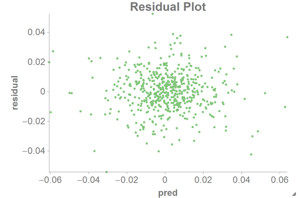

    

    For a residual plot, you want the distribution of points to be random, as in the chart above. If the distribution looks like a quadratic line or other non-linear form, you would probably need to transform your data in some way (e.g., using a log or square root function first).

    As a comparison, you can also create a scatter chart with eu as the x-axis and residual as the y-axis: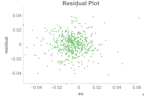

    

12. To see how good our fit is, you might want to plot the predicted value against the original response.

    Create a scatter chart with the predicted value (pred) as the x-axis and the original response (ise2) as the y-axis.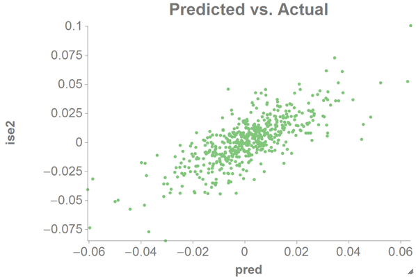

    

    This should look fairly linear if our estimation is good.

13. Another useful visualization is the QQ plot, which shows the relationship between the theoretical quantile and the sample quantile.

    <note>QQ plot</note>
    <tabu label="Tabulation on Istanbul" breaks="residual">
    <tcol source="residual" fun="cnt" name="count" label="Count"/>
    </tabu>
    <sort col="residual" dir="up"/>
    <willbe name="residual_cdf" value="g_cumsum(;;;count)/g_sum(;;count)" format="dec:7"/>
    <willbe name="theoretical_quantile" value="normal_cdf_inv(residual_cdf;0;1)" format="dec:7"/>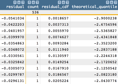

    

    We can then chart the QQ plot as a scatter chart in 1010data using the theoretical quantile (theoretical_quantile) as the x-axis and the sample quantile (residual) as the y-axis.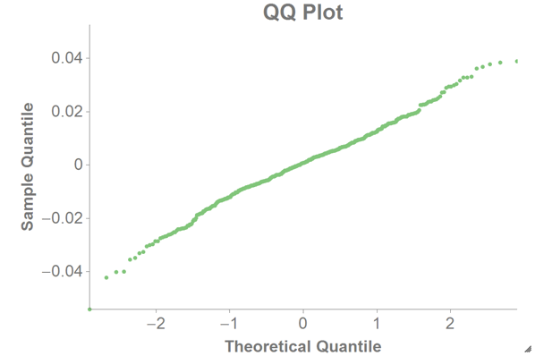

    

    We assume the residual follows a Gaussian distribution, in which case the QQ plot should be a straight line (as in the chart above). If the QQ plot is not a straight line, one should be careful when doing calculations using normal assumptions like confidence intervals or p-values.

14. You might also want to see the PP plot, which shows the theoretical cumulative probability vs. the sample cumulative probability.

    <note>PP plot</note>
    <note>The tabulation and sort from the previous step would go here if the previous step was not performed.</note>
    <willbe name="sample_cumulative_distribution" value="g_cumsum(;;;count)/g_sum(;;count)"/>
    <willbe name="resi_sd" value="sqrt(g_var(;;residual))"/>
    <willbe name="theoretical_cumulative_distribution" value="normal_cdf(residual;0;resi_sd)"/>

    Note: The <tabu> and <sort> operations from the previous step (QQ plot) need to have been performed before these <willbe> operations.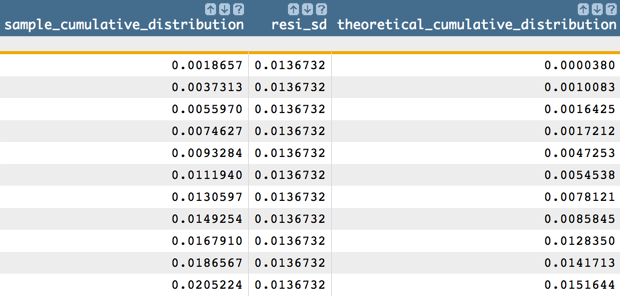

    

    We can then chart the PP plot as a scatter chart in 1010data using the theoretical cumulative probability (theoretical_cumulative_distribution) as the x-axis and the sample cumulative probability (sample_cumulative_distribution) as the y-axis.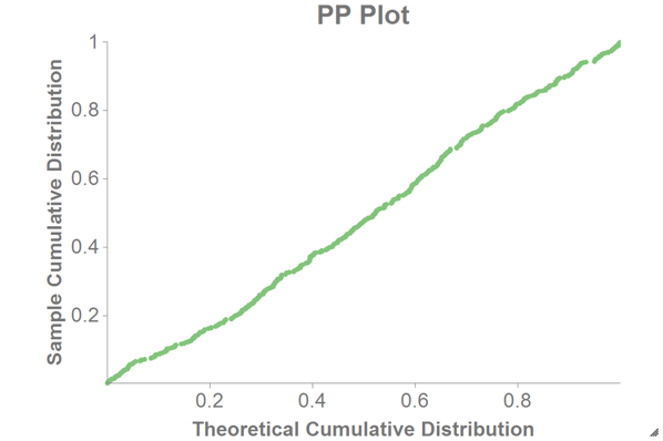

    

    If the normal assumptions hold, the PP plot should be a straight line (as in the chart above).