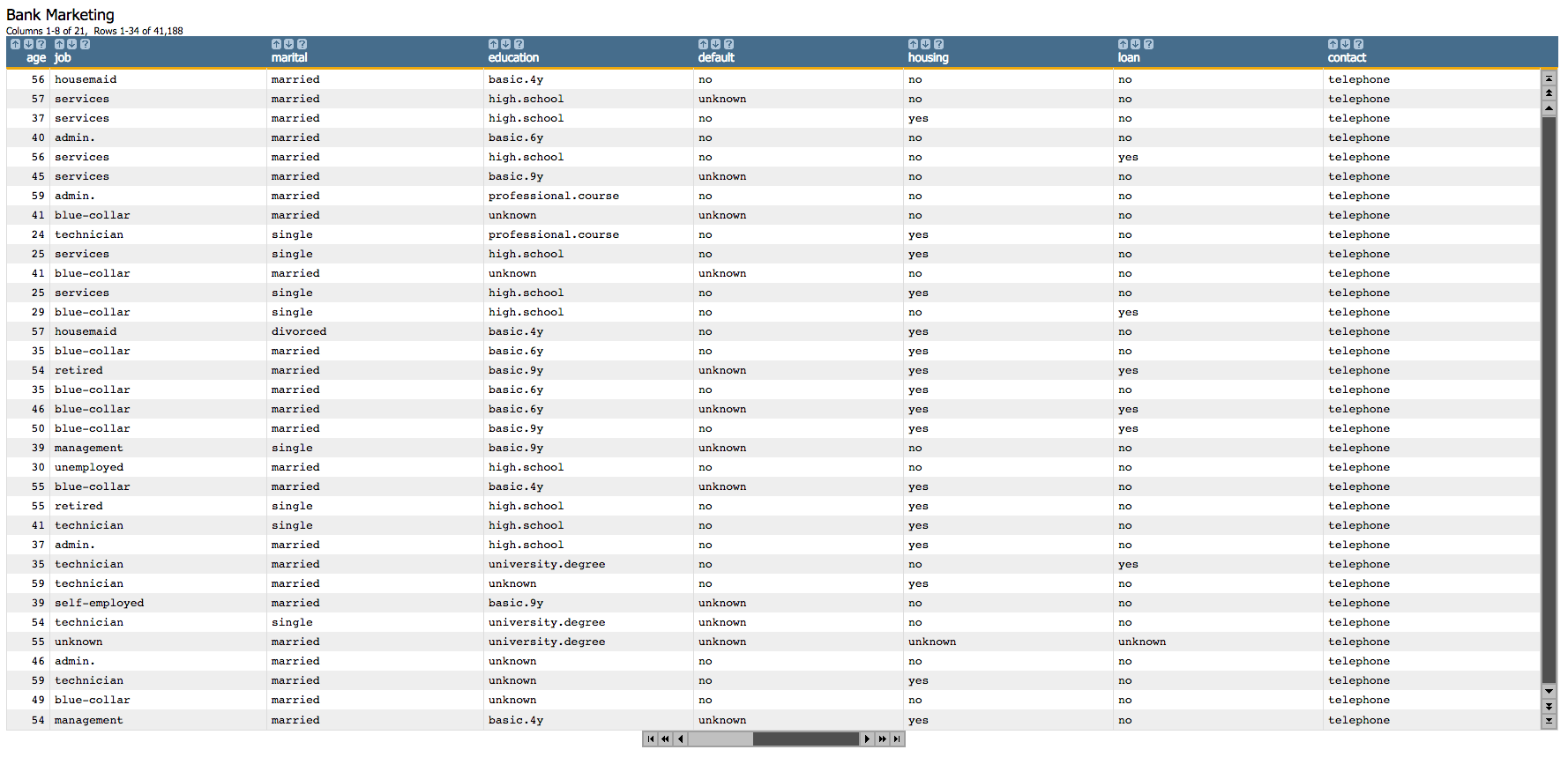
In this example, a logistic regression is performed on a data set containing bank
marketing information to predict whether or not a customer subscribed for a term
deposit.
The logistic regression, using the 1010data function g_logreg(G;S;Y;XX;Z), is applied to
the Bank Marketing Data Set, which contains information related to a campaign
by a Portuguese banking institution to get its customers to subscribe for a term deposit.
The logistic regression uses the following 10 variables in that data set as
predictors:
agedurationpreviousempvarratehousingdefaultloanpoutcomejobmarital
As a response, the column y is used, which is
yes if a customer has subscribed for a term deposit.
This analysis will follow the following steps:
- Prepare the data by creating dummy variables for each of the categorial
columns (since we cannot use textual data to build our model).
- Divide the data into a training set and a test set.
- Run the logistic regression on the training data set based on the continuous
variables in the original data set and the dummy variables that we
created.
- Obtain the predicted probability that a customer has subscribed for a term
deposit.
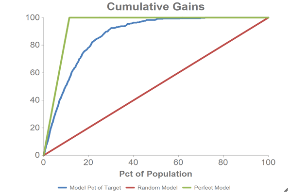
- Create a cumulative gains chart and calculate the area under the curve (AUC)
for the test data.
- Obtain the model coefficients.
- Chart the logistic curve for both the training and test data.
-
Open the Bank Marketing data set
(pub.demo.mleg.uci.bankmarketing).
-
Since we cannot use textual data in our analysis, we first create dummy
variables for each of the categorial columns.
<willbe name="yy" value="y='yes'"/>
<willbe name="hsng" value="housing='yes'"/>
<willbe name="h_unk" value="housing='unknown'"/>
<willbe name="def" value="default='yes'"/>
<willbe name="d_unk" value="default='unknown'"/>
<willbe name="loans" value="loan='yes'"/>
<willbe name="l_unk" value="loan='unknown'"/>
<willbe name="nonxst" value="poutcome='nonexistent'"/>
<willbe name="succ" value="poutcome='success'"/>
<willbe name="blue" value="job='blue-collar'"/>
<willbe name="tech" value="job='technician'"/>
<willbe name="j_unk" value="job='unknown'"/>
<willbe name="svcs" value="job='services'"/>
<willbe name="mgmt" value="job='management'"/>
<willbe name="ret" value="job='retired'"/>
<willbe name="entr" value="job='entrepreneur'"/>
<willbe name="self" value="job='self-employed'"/>
<willbe name="maid" value="job='housemaid'"/>
<willbe name="unemp" value="job='unemployed'"/>
<willbe name="stud" value="job='student'"/>
<willbe name="marr" value="marital='married'"/>
<willbe name="sgl" value="marital='single'"/>
<willbe name="m_unk" value="marital='unknown'"/>
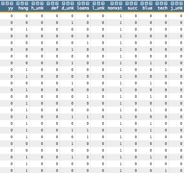
These <willbe>
operations create a computed column for each of the categories, where a
1 in the column indicates that the category
is true for that row. For instance, in the following screenshot, the rows
where hsng=1 indicate that the
client had a housing loan (i.e.,
housing='yes' in the original
table), and the rows where
h_unk=1 indicate that it
is unknown if the client had a housing loan (i.e.,
housing='unknown').

See Dummy Variables for a list of the dummy variables used here and their meanings.
-
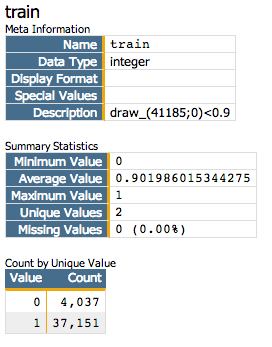
Next, we want to create a column that we will use to separate training data and
test data. We want to use 90% of our data as training data.
<note>SELECT TRAINING DATA</note>
<willbe name="train" value="draw_(41185;0)<0.9"/>
<willbe name="test" value="train<>1"/>
-
Now we run the logistic regression based on the continuous variables in the
original data set and the dummy variables that we created. We use the
train column from the previous step as the second parameter
of the g_logreg(G;S;Y;XX;Z)
function. The train column will act as a selector, so that our
function will only train 90% of the data. We also specify options for the
Z parameter that control convergence criteria.
<willbe name="model" value="g_logreg(;train;yy;1 age duration
previous empvarrate hsng h_unk def d_unk loans l_unk nonxst succ blue
tech j_unk svcs mgmt ret entr self maid unemp stud marr sgl m_unk;
'cgdeveps' 0.0000001 'lreps' 0.000000001)"/>
Note: The first element of XX
must be the special value 1 for the
constant (intercept) term in the linear model.
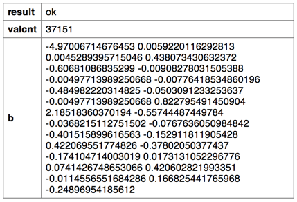
This creates a column named model that contains the results
of the logistic regression:

Clicking on the > opens a window containing a summary of the
model output:

-
We can then use the
score(XX;M;Z)
function to obtain the predicted probability (prob_score)
returned by the logistic model, which in our example represents the probability
a person subscribed for a term deposit.
<note>OBTAIN MODEL SCORE WITH SCORE FUNCTION</note>
<willbe name="prob_score" value="score(1 age duration previous empvarrate
hsng h_unk def d_unk loans l_unk nonxst succ blue tech j_unk svcs mgmt ret
entr self maid unemp stud marr sgl m_unk;model;)" format="dec:7"/>
Note: We specify format="dec:7" so that our results show
with 7 decimal places.
-
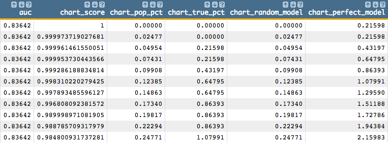
To create the cumulative gains chart and calculate the area under the curve,
clone the current tab and follow the
steps in Chart cumulative gains and calculate the AUC in the cloned tab.
You should see results similar to the
following:


-
To obtain the model coefficients, we can use the
param(M;P;I)
function. For our example, we will only obtain the parameters for the intercept
(b0) and the first three variables (b1,
b2, and b3).
Note: Perform the remaining steps in the original tab, not the cloned
tab.
<willbe name="b0" value="param(model;'b';1)" format="dec:7"/>
<willbe name="b1" value="param(model;'b';2)" format="dec:7"/>
<willbe name="b2" value="param(model;'b';3)" format="dec:7"/>
<willbe name="b3" value="param(model;'b';4)" format="dec:7"/>
-
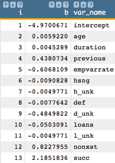
One might also want to obtain coefficients in one column, which can be achieved
with the following:
<note>CALCULATE COEFFICIENTS IN ONE COLUMN</note>
<willbe name="var_names" value="'intercept,age,duration,previous,
empvarrate,hsng,h_unk,def,d_unk,loans,l_unk,nonxst,succ,blue,tech,
j_unk,svcs,mgmt,ret,entr,self,maid,unemp,stud,marr,sgl,m_unk'"/>
<willbe name="temp_i" value="mod(i_(1);27)"/>
<willbe name="i" value="if(temp_i=0;27;temp_i)"/>
<willbe name="b" value="param(model;'b';i)" format="dec:7"/>
<willbe name="var_name" value="csl_pick(var_names;i)"/>

Note: The number of coefficients we obtain from the model corresponds to the
number of variables in our analysis. So, for our example, we obtain 27
coefficients (the intercept and the 26 predictors).
-
To extract logistic regression fit statistics (e.g., deviance, AIC, p-values,
z-values, and standard errors), clone the current tab and follow the
steps in Extract logistic regression fit statistics in the cloned tab.
A number of new columns containing the various
fit statistics (as well as some intermediary columns that are used in the
calculation of the fit statistics) will be added to the table.
For example, the following columns show deviance and AIC:

The columns below show the standard error, z-values, and p-values for both
the intercept (indicated by const in the column names) and
the age variable:

-
We can also calculate the logit of the predicted probability
(
prob_score), which we can use for purposes of further
analysis such as visualization.
Note: Perform the remaining steps in the original tab, not the cloned
tab.
<willbe name="z_estimate" value="loge(prob_score / (1-prob_score))" format="dec:7"/>
-
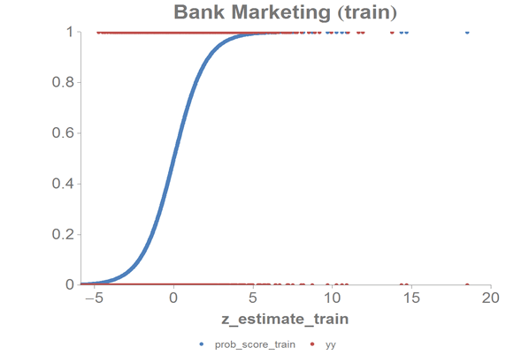
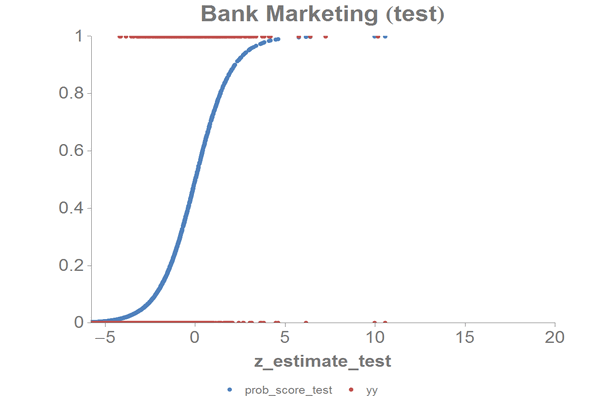
We can chart the logistic curve for both the training and test data using the
1010data Chart Builder.
Let's chart the results for our training data:
-
Create computed columns that contain the
prob_score
and z_estimate for just the training data.
<willbe name="prob_score_train" value="prob_score*train"/>
<willbe name="z_estimate_train" value="z_estimate*train"/>
-
Click .
-
Drag the
z_estimate_train column to the
DATA (X-AXIS) area.
-
Drag the
prob_score_train and yy
columns to the DATA (Y-AXIS) area.
-
Change X-Range (max) to
20.
-
Click Update.
Let's chart the results for our test data:
-
Create computed columns that contain the
prob_score
and z_estimate for just the test data.
<willbe name="prob_score_test" value="prob_score*test"/>
<willbe name="z_estimate_test" value="z_estimate*test"/>
-
Click .
-
Drag the
z_estimate_test column to the DATA
(X-AXIS) area.
-
Drag the
prob_score_test and yy
columns to the DATA (Y-AXIS) area.
-
Change X-Range (max) to
20.
-
Click Update.
The results should look similar to the following charts:
