Creating a simple pivot table

Performing a cross tabulation can produce a table that mimics a pivot table in Excel.

Difficulty

Objective

You would like to aggregate a large amount of data and have the results shown over two metrics in a new table. For example, you have a data set consisting of completed sales transactions for a given time period and you would like a table that shows the sum of sales for each individual store and each department within each store. You know how to create a pivot table in Excel and you want to obtain the same results using 1010data.

Excel solution

Pivot tables in Excel are useful because they allow you to summarize large amounts of data and view it across multiple metrics. Additionally, Excel's user-friendly GUI allows you to easily manipulate the data to properly fit your desired table.

After selecting a cell inside your data set, you can insert a pivot table based on the data associated with that cell.

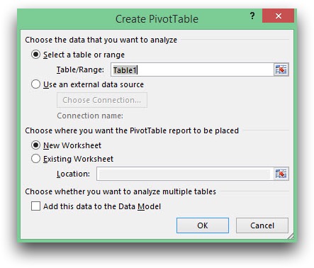
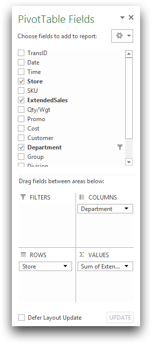
Your pivot table will be created in a new worksheet, or the existing worksheet, based on your selection. You can then use the GUI to drag which data you want to be displayed as columns and rows, and which data you want to be summarized.

Your completed pivot table should look like the sample below.

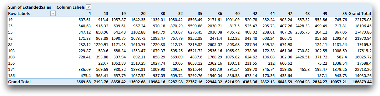
Although the process to create a pivot table in Excel is relatively simple, it has its limitations. The original table containing sales transactions is too large for Excel to process, therefore these calculations are only done on a subset of the data.

Instead, if you use 1010data's platform to perform the same operation, there is a much larger limit to the size of your data. Additionally, 1010data also has an easy to use GUI to produce an Excel like pivot table using a cross tabulation.

1010data GUI solution

Upon opening the Sales Detail table, click Analysis > Cross Tabulation to open the dialog shown below.

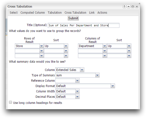
Here you can see some similarities to Excel's GUI. However, instead of dragging the desired data, you use the drop-down menus, to select the data for the rows and columns of the cross tabulation or "pivot table." You also select the data for which to summarize, and the type of summary you wish to complete. There are additional options you can utilize such as the sort direction and adding a reference column.

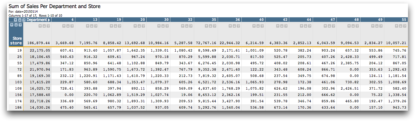
For this analogue, Store is selected from the first Rows of Result drop-down menu and Department from Columns of Result. You want to compute the sum sales over these metrics, therefore you select Extended Sales for the column that contains the summary data and sum for the Type of Summary. After selecting these inputs and clicking Submit, you obtain the table below.

1010data Macro Language solution

You can obtain the same result in 1010data's platform by entering the macro code into the Edit Actions dialog instead of using the GUI. Below is the macro code that creates the pivot table-like results.

<base table="pub.doc.retail.altseg.sales_detail_transid"/>
<sel value="trans_date=20150114"/>
<tabu label="Sum of Sales Per Department and Store" 
 breaks="store" cbreaks="dept" clabels="short">
  <break col="store" sort="up"/>
  <break col="dept" sort="up"/>
  <tcol source="xsales" fun="sum"/>
</tabu>

The selection of data is completed in order to effectively mimic the Excel pivot table, which can only compute a subset of the data due to size limitations. However, 1010data can complete the aggregation on the entire data set. The <tabu> operation contains attributes that establish the title of the new table, as well as what data to group the rows and columns by. Within this operation, child elements are contained. <break> specifies the sort direction for a grouping column, and <tcol> specifies the source column to summarize and the summary function that will be used on that column. The resultant table can be seen below.