g_markov(G;S;O;T;H;D;M)
Returns the results of running a Monte Carlo Markov-chain simulation within a given group.
Syntax
g_markov(G;S;O;T;H;D;M)Input
| Argument | Type | Description | |||||||||
|---|---|---|---|---|---|---|---|---|---|---|---|
G |
any | A space- or comma-separated list of column names Rows are in the same group
if their values for all of the columns listed in If If any of the columns listed in |
|||||||||
S |
integer | The name of a column in which every row evaluates to a 1 or 0, which determines
whether or not that row is selected to be included in the calculation If
If any of the values in
|
|||||||||
O |
integer | A space- or comma-separated list of column names that
determine the row order within a particular group If
If any of the values in |
|||||||||
T |
integer | A scalar value or the name of a column
If present, T
must be (within each group) a non-decreasing sequence of integers greater than or
equal to zero. For example: 1,2,3,4... or 0,1,4,5,5,6,7...
If the sequence begins with 0, then the state at that row is the initial state
(see If
|
|||||||||
H |
integer | A scalar value or the name of a column
If |
|||||||||
D |
integer | A scalar value or the name of a column
If
|
|||||||||
M |
decimal | A space- or comma-separated list of either
scalar values or column names
For example, the list:
represents the 3*3 matrix:
The value in row I, column J is to be interpreted as the probability that state I will transition to state J. The values in each row should sum to 1.0 (if they
do not, the result from |
T, H, D, and M
are the same, then the result of g_markov will be the same (for the same
number of rows).Return Value
For every row in each group defined by G (and for those rows where
S=1, if specified), g_markov
returns an integer value corresponding to the state with respect to running a Monte Carlo
Markov-chain simulation within that group, where the order of rows in the simulation is
determined by O, if specified (otherwise, the order is the current display
order of the table).
The simulation starts at a state H, and at each time step
T, "the dice are rolled" and the next state is transitioned to with a
probability determined by M. The result of the function for each row is the
state at that row.
Example
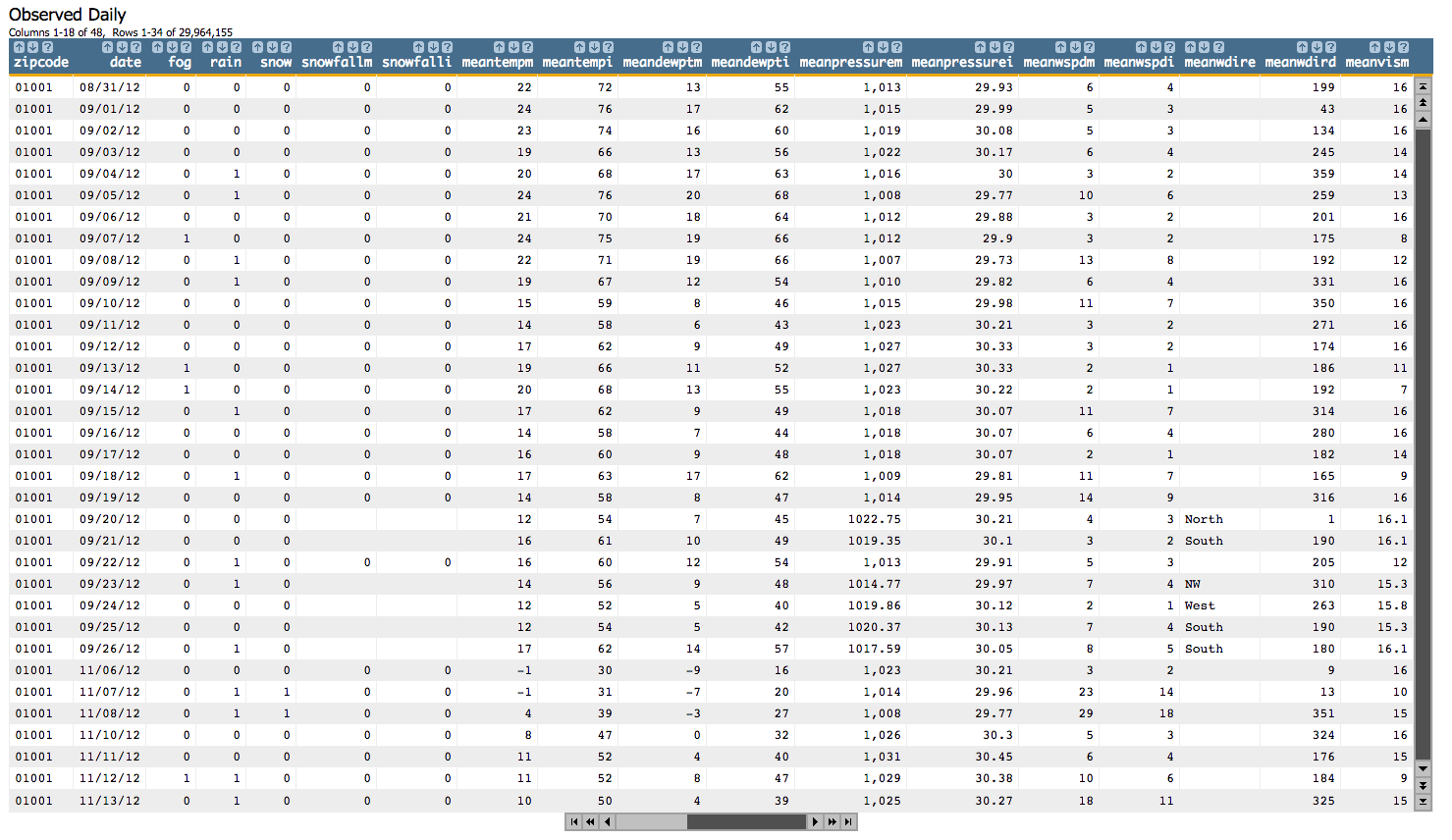
Let's use the Weather Underground Observed Daily table
(pub.demo.weather.wunderground.observed_daily) to illustrate the use
of g_markov(G;S;O;T;H;D;M).
Let's say we want to perform a Monte Carlo Markov-chain simulation to generate random samples of weather conditions in a particular zip code. To do this, we'll need a transition matrix that consists of the probabilities of weather conditions for that zip code, specifically related to sunny vs. rainy days.
Our transition matrix should look something like:
probS_S |
probS_R |
probR_S |
probR_R |
probS_Sis the probability that it will be sunny tomorrow given that it is sunny todayprobS_Ris the probability that it will be rainy tomorrow given that it is sunny todayprobR_Sis the probability that it will be sunny tomorrow given that it is rainy todayprobR_Ris the probability that it will be rainy tomorrow given that it is rainy today
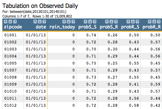
We can easily figure out this matrix from the data in the table by using the following Macro Language code:
<sel value="between(date;20130101;20140101)"/>
<tabu label="Tabulation on Observed Daily" breaks="zipcode,date">
  <break col="date" sort="up"/>
  <tcol source="rain" fun="hi" name="rain" label="Highest`Rain``"/>
</tabu>
<willbe name="rain_today" value="int(rain)"/>
<willbe name="sunny_today" value="~rain_today"/>
<willbe name="rain_tomorrow" value="g_rshift(zipcode;;;rain_today;1)"/>
<willbe name="probR_R" value="g_sum(zipcode;rain_today;rain_tomorrow)/g_sum(zipcode;;rain_today)" format="dec:2"/>
<willbe name="probR_S" value="1-probR_R" format="dec:2"/>
<willbe name="probS_R" value="g_sum(zipcode;sunny_today;rain_tomorrow)/g_sum(zipcode;;sunny_today)" format="dec:2"/>
<willbe name="probS_S" value="1-probS_R" format="dec:2"/>
<colord cols="zipcode,date,rain_today,probS_S,probS_R,probR_S,probR_R"/>
This will give us the following results:
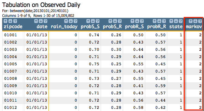
For g_markov(G;S;O;T;H;D;M), we'll specify zipcode for
the G parameter, since we want to run the simulation for each zip code.
We'll omit the S parameter since we want the function to consider all rows
and not just a subset, and we'll specify date for the O
parameter to order the rows in the simulation by date.
We'll omit the T parameter, so that the result in each of the rows will
represent a single step in the simulation.
H parameter, we need to specify a start state, which can either be
1 (sunny) or 2 (rainy), so we'll create a
state column we can use for that
parameter:<willbe name="state" value="rain_today+1"/>For the D parameter, we need to specify an integer value that will
determine the random seed for the group. For our example, we'll use the value
42, but this can be any integer value.
Finally, the M parameter would be the list of values from our transition
matrix: probS_S probS_R probR_S probR_R.
g_markov(G;S;O;T;H;D;M) would look
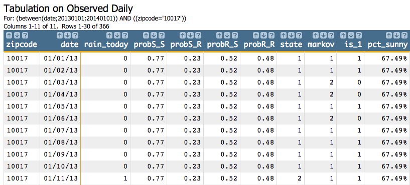
like:<willbe name="markov" value="g_markov(zipcode;;date;;state;42;probS_S probS_R probR_S probR_R)"/>This gives us results similar to the following:
<sel value="(zipcode='10017')"/>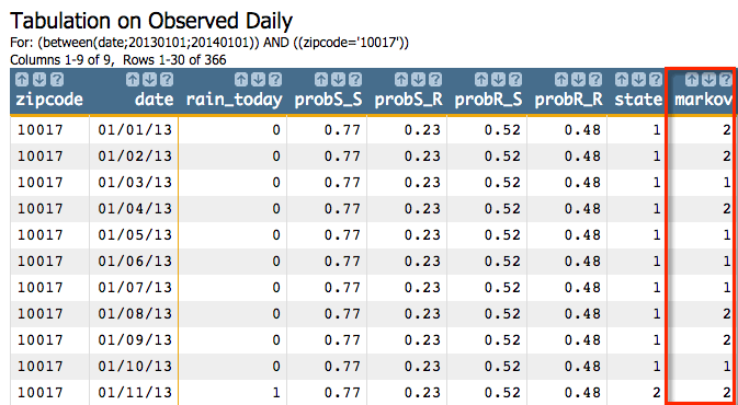
Since we ordered by the date column, the simulation will start at the row
with the date 01/01/13, and the start state will be
1. The result from the first step of the simulation using the seed
and the transition matrix we specified, is 2, which becomes the
start state for the next step of the simulation. The result from that step is
2, and then 1, and so on for all
366 steps of the simulation.
<willbe name="is_1" value="markov=1"/>
<willbe name="pct_sunny" value="g_cnt(zipcode;is_1)/g_cnt(zipcode;)" format="type:pct;dec:2"/>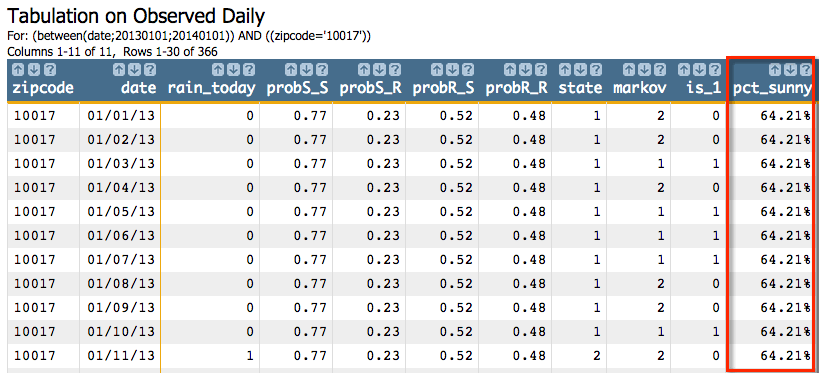
So we can see that 64.21% of the time in this simulation,
g_markov predicted the weather would be sunny. If we ran the simulation
with a different seed or ran it on a different zip code that had a different transition
matrix, we would get slightly different results. For example, if we changed the seed to
38746 for the 10017 zip code, we would get
the following results: