Incorporating a dynamic drop-down in the dashboard
The contents of dynamic drop-downs can change based on selections in the dashboard or the results of queries.
Dynamic drop-down lists means your dashboard will always be up to date even as the data changes. This is difficult to achieve using Excel alone.
Let's take a look at how to create a dynamic drop-down. Our original query calculated the sum of sales for one particular department, which was hard-coded into the query. Let's say we want to give the user of our dashboard the ability to select the department from a list of all the departments in our Product Master table. We could go through that table and list each department individually like we did in the previous step, Creating a static drop-down in the dashboard, but since our Product Master table has 59 different departments, that would be a bit time consuming and could introduce errors (for instance, if a department number was entered incorrectly). It would be easier (and less susceptible to error) if we ran a simple query on the Product Master table to find out the list of departments in the table and then used those results as the items in the drop-down. Let's create a dynamic drop-down to do just that.
We'll need to write a query that gives us a list of all the departments in the Product Master table, and we'll need to put the results of that query in a place that our dashboard can access. We'll also need to create the actual drop-down on the dashboard and populate it with the results of our department list query.
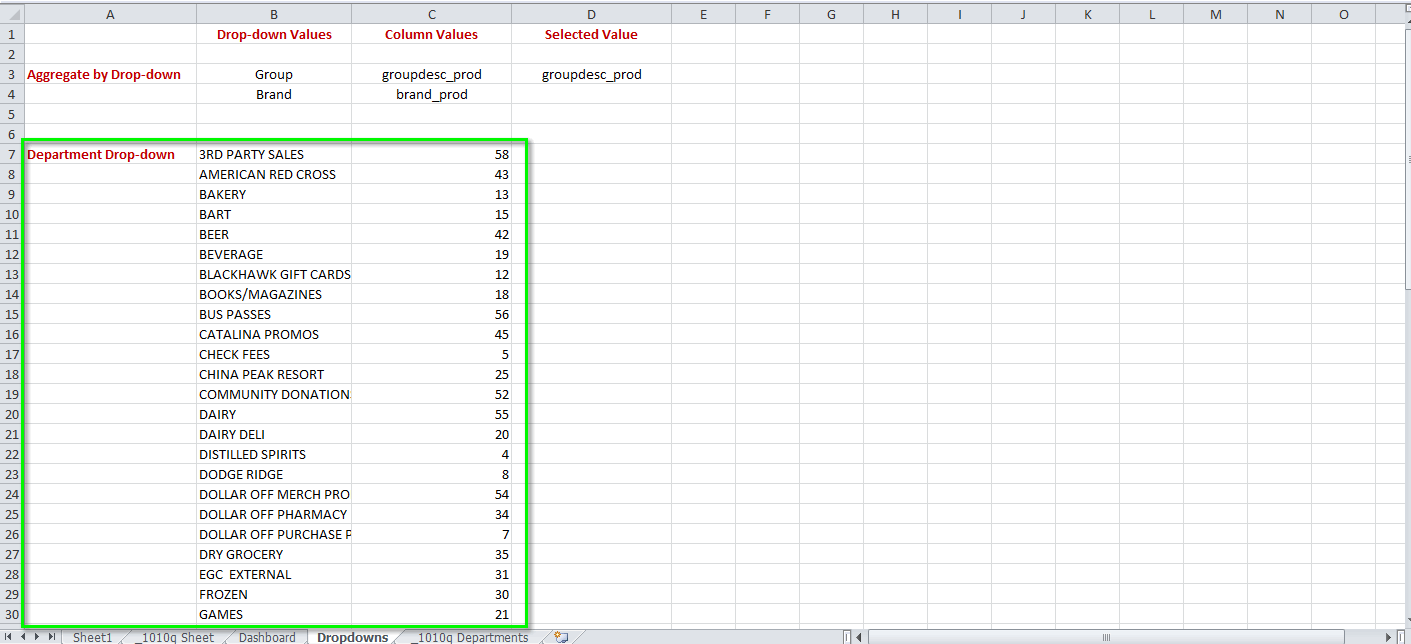
Since we already have a worksheet that we use for holding the values in our Aggregate by drop-down, let's use that same worksheet to hold the values for our dynamic drop-down. Click on the Dropdowns tab and enter a label similar to the one shown in cell A7 below. Then click in the cell where you want the results pasted, which in our example is B7, and give it a defined name. Let's call it dept_list.
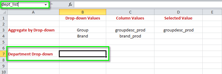
Now that we have a destination for the results of our query, let's create the query.
We'll need to create another q-sheet, since each q-sheet can only contain one query.
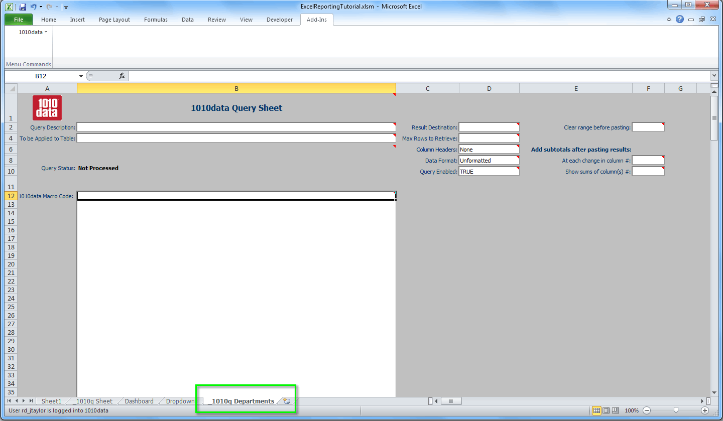
<ignore type="base">Applied to table: retaildemo.products</ignore>
<tabu label="Tabulation on Product Master" breaks="deptdesc,dept">
  <break col="deptdesc" sort="up"/>
  <tcol source="deptdesc" fun="cnt" label="Count"/>
</tabu>
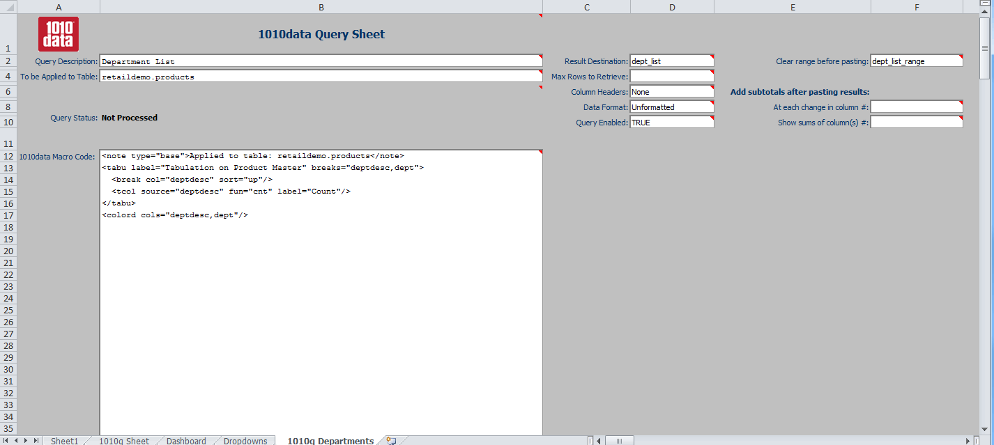
<colord cols="deptdesc,dept"/>- For the Query Description, enter "Department List".
- In the To be Applied to Table field, we need to specify which table this query should be applied to. For this q-sheet, we'll enter retaildemo.products.
- In the Result Destination field, enter dept_list so that the results of our query will be pasted in the Dropdowns worksheet.
- From the Column Headers drop-down, select "None", which is the default. We don't need any column headers since the results of the query are going to be used to populate the drop-down.
Finally, before we paste the results of the query, let's clear the contents from any previous run. Create a defined name for the range of cells where the results will be pasted. On the Formulas tab, click Define Name. In the New Name dialog, enter dept_list_range for the Name and enter the following for Refers to: =Dropdowns!$B$7:$C$500.
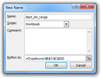
Then, in the _1010q Departments q-sheet, we can enter dept_list_range in the Clear range before pasting field.
Our q-sheet should look similar to the following:
To run the q-sheet, click , or press Ctrl+Q.
To see the results, click the Dropdowns tab. You can see that the results of the query have been pasted in the cells that we specified:
Let's create the drop-down on our dashboard and use these values to populate it. Click on the Dashboard tab and add a label where you want the drop-down to appear:
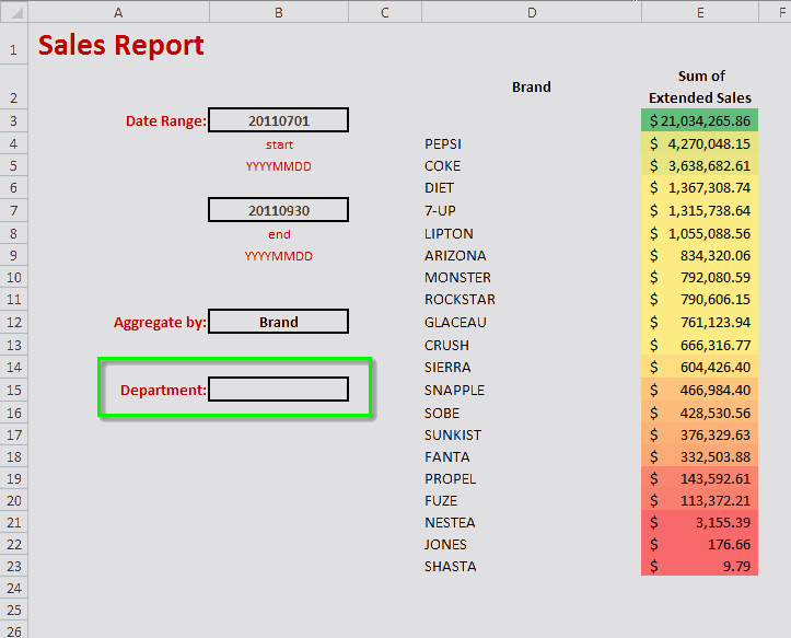
Click the cell that will contain the drop-down. In our example, that would be cell B15. Let's also give it the defined name: department_dropdown.
OFFSET
function:=OFFSET(dept_list_range,0,0,COUNTA(dept_list_range),1)dept_list_range), and the
second and third parameters tell the OFFSET function to start the list with
the top left value in that range. The fourth parameter uses the Excel COUNTA function to calculate the
number of non-empty cells in the range, which in essence specifies the length of the list. The
last parameter tells the OFFSET function that we just want one column of data
from the results. Dynamic drop-downs require this OFFSET function in
conjunction with the COUNTA function to automatically account for the varying
length of the list returned from our query. So, our Data Validation
dialog will look something like: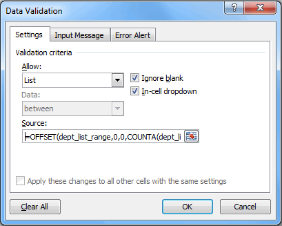
Click OK in the Data Validation dialog to finish creating the drop-down.
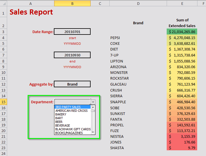
Now, if you click the newly created drop-down, you should see the list of all the departments returned by the query in the _1010q Departments q-sheet:
20 in the value attribute to the <sel> operation. Right now, it's
hard-coded to be
19:<ignore type="base">Applied to table: retaildemo.salesdetail</ignore>
<sel value="between(date;20110101;20110331)"/>
<link table2="retaildemo.products" col="sku" col2="sku" suffix="_prod" type="select">
<sel value="(dept=19)"/>
</link>
<tabu label="Tabulation on Sales Detail" breaks="groupdesc_prod">
<tcol source="xsales" fun="sum" name="tot_sales" label="Sum of`Extended Sales"/>
</tabu>
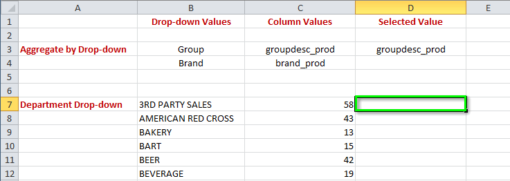
<sort col="tot_sales" dir="down"/>So let's go back to the Dropdowns worksheet and choose a cell that will contain the department value associated with the selected item in the Department drop-down (similar to what we did in Creating a static drop-down in the dashboard). For our example, we'll use cell D7. Let's give that cell the defined name department_selected.
VLOOKUP() to help us do that. Let's add the
following formula to cell
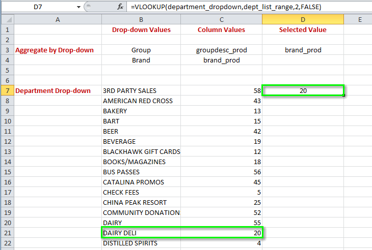
D7:=VLOOKUP(department_dropdown,dept_list_range,2,FALSE)This says that for the value in the cell named department_dropdown, search
the first column in the table defined by the range dept_list_range, and
return the value in the second column, and only return if there is an exact match (which there
will always be since we populated the drop-down from this list). So, if the user selects
"DAIRY DELI" from the drop-down in the Dashboard
worksheet, the VLOOKUP function will search the values in the
Drop-down Values column on the Dropdowns
worksheet until it finds a match, and then return the value in the Column
Values column, which for our example is 20:
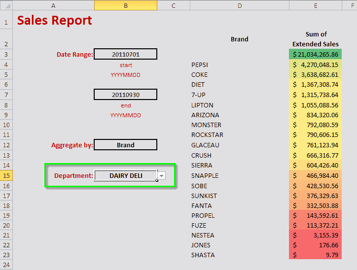
The last step is to reference the selected value in our original query. This process is essentially the same as what we did in Adding a static input to a dashboard and Creating a static drop-down in the dashboard.
<ignore type="base">Applied to table: retaildemo.salesdetail</ignore>
<sel value="between(date;20110101;20110331)"/>
<link table2="retaildemo.products" col="sku" col2="sku" suffix="_prod" type="select">
  <sel value="(dept=19)"/>
</link>
<tabu label="Tabulation on Sales Detail" breaks="groupdesc_prod">
  <tcol source="xsales" fun="sum" name="tot_sales" label="Sum of`Extended Sales"/>
</tabu>
<sort col="tot_sales" dir="down"/>- removing any blank spaces from the start of the line
- inserting an = at the beginning of the line
- enclosing the macro code in double quotes
- preceding any double quote within the macro code with another double quote so that Excel will not interpret any of them as the end of the formula
- replacing each hard-coded value with a reference to its corresponding input cell using the syntax: "&[CELL_REFERENCE]&" (e.g., "&B3&")
Let's go through those steps for our example. Click on the _1010q Sheet tab so that we can modify the macro code in our q-sheet.
<sel value="(dept=19)"/>=<sel value="(dept=19)"/>="<sel value="(dept=19)"/>"="<sel value=""(dept=19)""/>"19 value with a
reference to the department_selected cell, which contains the value the
user selected from the
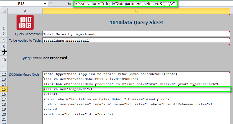
drop-down:="<sel value=""(dept="&department_selected&")""/>"&department_selected&
for this Excel formula to work properly.Now we can see the line in our macro code consists of the formula we just created and that it
resolves to 20 within the 1010data Macro Code section
of the q-sheet:
Now let's test this out. Click (or press Ctrl+Q).
When the query completes, you can see that the results show the sum of extended sales for each brand in department 20:
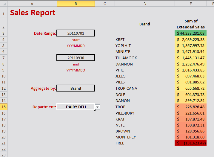
You can also see that the cell for the last item in the list, which contains a negative value, appears with a dark red fill color, which we specified in Conditional Formatting.
