
Creating a static drop-down in the dashboard
Let's create a drop-down to give the users of our dashboard the ability to select, from a static set of values, the column by which they want to group the results of the tabulation.
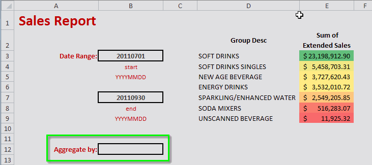
Currently, our query tabulates the sum of extended sales, grouping by the values in the Group Desc column in the Product Master table. Let's make it so that the user can select to group the results of the tabulation either by the group description or by the brand.
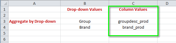
We're going to need a place to list the values that will populate the static drop-down. We can use Sheet3 for our drop-down values (or create a new worksheet, if necessary). Let's rename it "Dropdowns".
In the Dropdowns worksheet, enter the following information:
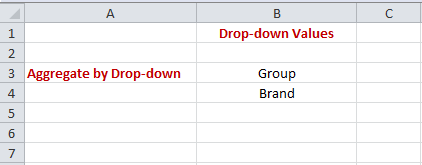
Let's give this range of values a defined name. On the Formulas tab, click Define Name. In the New Name dialog, enter aggregate_by_values for the Name and enter the following for Refers to: =Dropdowns!$B$3:$B$4, then click OK.
Now let's go back to the Dashboard tab and create the static drop-down.
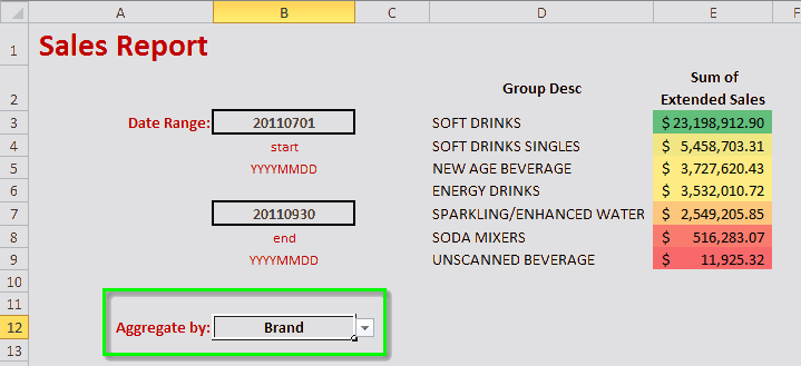
In the Dashboard worksheet, add the label "Aggregate by:" next to where you want the drop-down to appear.
Click the cell that you want to contain the drop-down. In our example, that would be cell B12. Let's give that cell the defined name aggregate_by_dropdown.
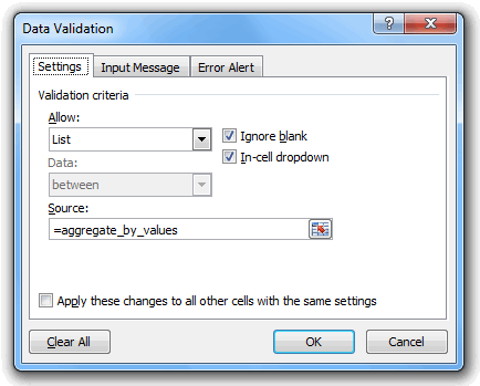
From the Data tab, click Data Validation. In the Data Validation dialog, select List from the Allow drop-down, and enter =aggregate_by_values in the Source field:
Then click OK in the Data Validation dialog to finish creating the drop-down.
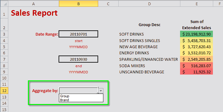
Now, if you click the newly created drop-down, you should see the two values, Group and Brand, in the list:
brand_prod for the breaks
attribute to the <tabu> operation. Right now, it's hard-coded
to be
groupdesc_prod:<ignore type="base">Applied to table: retaildemo.salesdetail</ignore>
<sel value="between(date;20110101;20110331)"/>
<link table2="retaildemo.products" col="sku" col2="sku" suffix="_prod" type="select">
<sel value="(dept=19)"/>
</link>
<tabu label="Tabulation on Sales Detail" breaks="groupdesc_prod">
<tcol source="xsales" fun="sum" name="tot_sales" label="Sum of`Extended Sales"/>
</tabu>
<sort col="tot_sales" dir="down"/>So let's go back to the Dropdowns worksheet and add another column that will associate the drop-down choices with their corresponding column names:
Since our query needs to reference a single cell (similar to what we did in Adding a static input to a dashboard), we also need somewhere to store the choice that the user makes from the drop-down. Let's add one more column to the Dropdowns worksheet with a cell that will hold that value:
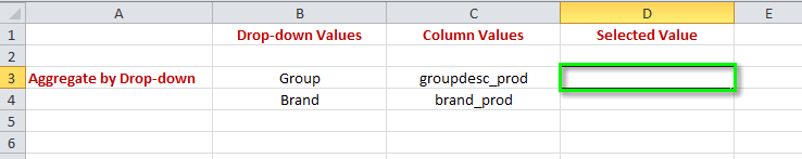
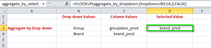
So, for our example, whatever choice the user selects from the drop-down will be stored in cell D3. Let's give that cell the defined name aggregate_by_selected
VLOOKUP() to help us do that. Let's add the
following formula to cell
D3:=VLOOKUP(aggregate_by_dropdown,'Dropdowns'!B3:C4,2,FALSE)This says that for the value in the aggregate_by_dropdown, search the
first column in the table defined by the range 'Dropdowns'!B3:C4, and return
the value in the second column (which we indicate by setting the third parameter to
2), and only return if there is an exact match, which we specify by
setting the last parameter to FALSE Keep in mind that there will always
be an exact match since we only have a finite number of defined choices in the drop-down.
So, if the user selects Brand from the drop-down in the
Dashboard worksheet, the VLOOKUP function will search
the values in the Drop-down Values column on the
Dropdowns worksheet and will return the value in the second column,
which is brand_prod:
Now that we have the column name, we can insert it into our query, just like we did in Adding a static input to a dashboard.
<ignore type="base">Applied to table: retaildemo.salesdetail</ignore>
<sel value="between(date;20110101;20110331)"/>
<link table2="retaildemo.products" col="sku" col2="sku" suffix="_prod" type="select">
  <sel value="(dept=19)"/>
</link>
<tabu label="Tabulation on Sales Detail" breaks="groupdesc_prod">
  <tcol source="xsales" fun="sum" name="tot_sales" label="Sum of`Extended Sales"/>
</tabu>
<sort col="tot_sales" dir="down"/>- removing any blank spaces from the start of the line
- inserting an = at the beginning of the line
- enclosing the macro code in double quotes
- preceding any double quote within the macro code with another double quote so that Excel will not interpret any of them as the end of the formula
- replacing each hard-coded value with a reference to its corresponding input cell using the syntax: "&[CELL_REFERENCE]&" (e.g., "&B3&")
Let's go through those steps for our example. Click on the _1010q Sheet tab so that we can modify the macro code in our q-sheet.
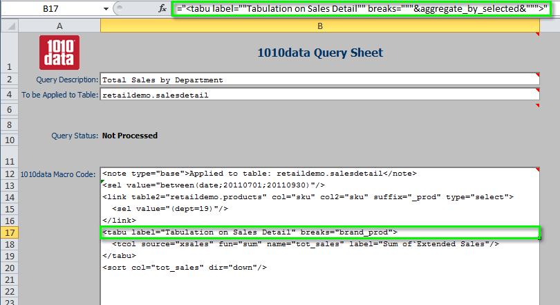
=<tabu label="Tabulation on Sales Detail" breaks="groupdesc_prod">="<tabu label="Tabulation on Sales Detail" breaks="groupdesc_prod">"="<tabu label=""Tabulation on Sales Detail"" breaks=""groupdesc_prod"">"groupdesc_prod value with a
reference to the aggregate_by_selected cell, which contains the value
the user selected from the
drop-down:="<tabu label=""Tabulation on Sales Detail"" breaks="""&aggregate_by_selected&""">"&aggregate_by_selected&.
Although this may look odd, it is correct syntax for this Excel formula to work
properly.We can see the line in our macro code now consists of the formula we just created and that it
resolves to brand_prod within the 1010data Macro Code
section of the q-sheet:
Now let's test this out. Click (or press Ctrl+Q).
When the query completes, click the Dashboard tab to see that the results show the sum of extended sales for each brand:
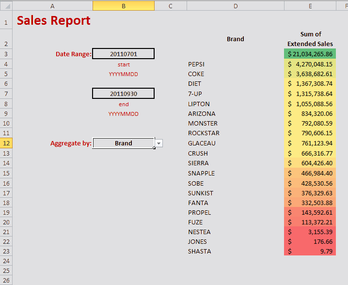
The results we see are for department 19 only, since that was the department that was hard-coded in our original query. The next step will show how to add a dynamic drop-down that allows the user to choose any department.