Perform a cross tabulation
A cross tabulation allows you to calculate, or summarize, the values in a column based on the values in two or more other columns and display the result as a matrix.
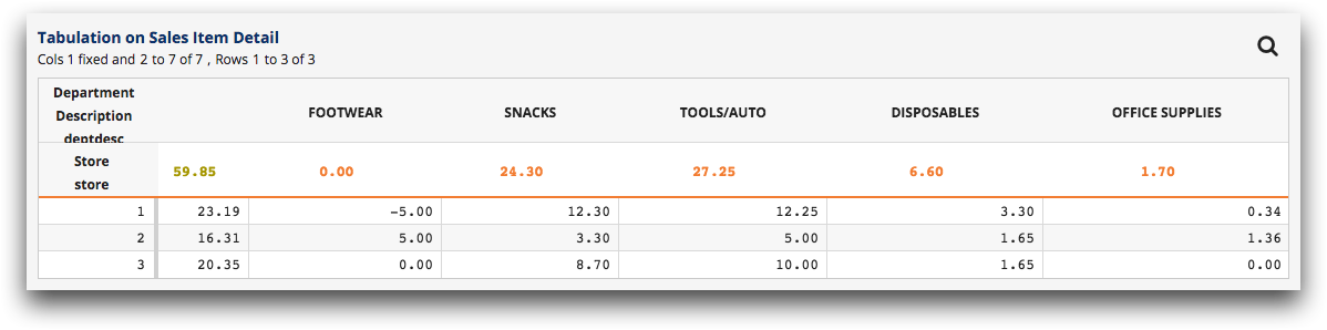
A cross tabulation can help you gain granularity from a summary without losing the highest level of data summarization. For example, in addition to finding the total amount of sales for each store in a grocery chain, you can also obtain the sales figures for the individual departments within each store and how they compare to the total.
To perform a cross tabulation:
-
In the New operation panel, click
Tabulate.
The Trillion-Row Spreadsheet displays the Tabulation panel.
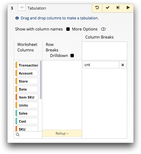 Note: By default, a new Tabulation panel contains the cnt (count) tabulation function.
 -
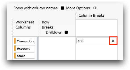
If applicable, remove the default tabulation function by clicking the
Delete Function (
 ) icon in
the field.
) icon in
the field.
-
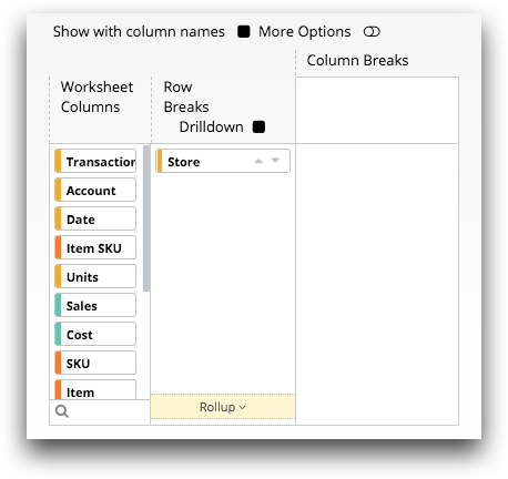
For the rows in the resultant cross tabulation,
specify each column by which you want to group the
data.
-
Drag the column from the Worksheet Columns
section to the Row Breaks section.
This selection groups the data by creating a separate row in the resultant worksheet for each unique value within the chosen column. Grouping is a way of pooling all the records for a single entity or value into a single entry in the worksheet.Note: In most cases, the order by which you choose to group the data is important because it can affect the results of the cross tabulation.The Trillion-Row Spreadsheet moves the column to the Row Breaks section.
-
Optionally, set the sort order of the column by either clicking the
Sort Up (
 ) or
Sort Down (
) or
Sort Down ( )
icon.
)
icon.
All rows that have the same values for all of the columns specified will be considered part of one group.
-
Drag the column from the Worksheet Columns
section to the Row Breaks section.
-
For the columns in the resultant cross
tabulation, specify each column by which you want to group the
data.
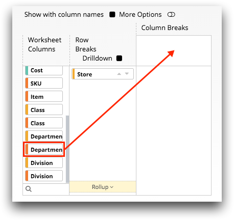
-
Drag the column from the Worksheet Columns
section to the upper area of the Column Breaks
section.
This selection groups the data by creating a separate column in the resultant worksheet for each unique value within the chosen column. Grouping is a way of pooling all the records for a single entity or value into a single entry in the worksheet.
 Note: In most cases, the order by which you choose to group the data is important because it can affect the results of the cross tabulation.The Trillion-Row Spreadsheet moves the column to the upper area of the Column Breaks section.
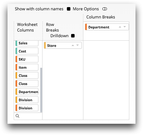
-
Optionally, set the sort order of the column by either clicking the
Sort Up () or
Sort Down ()
icon.
All rows that have the same values for all of the columns specified will be considered part of one group.
-
Drag the column from the Worksheet Columns
section to the upper area of the Column Breaks
section.
-
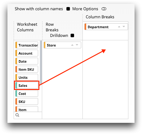
For each column of data that you want to summarize, complete the
following:
-
Drag the column from the Worksheet Columns
section to the lower area of the Column Breaks
section.
This selection chooses the column of data you want to summarize.
 The Trillion-Row Spreadsheet adds a tabulation function field and returns the column to the Worksheet Columns section.Note: By default, columns placed in the lower area of the Column Breaks section are assigned the sum of [COLUMN] summarization. If the data type of the column is text, it is assigned the last of [COLUMN] summarization.
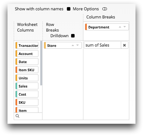
-
Drag the column from the Worksheet Columns
section to the lower area of the Column Breaks
section.
-
Optionally, create a drilldown analysis from the cross tabulation
results.
A drilldown analysis provides an interactive way to explore data points and view row-level data in the grid without changing your underlying query. For instructions, see Set up a drilldown hierarchy.
t0, t1, t2, and so on, for
each summarization column and m0, m1,
m2, and so on, for each tabulated column break. You can give
the resultant columns more meaningful names within the More
Options view of the Tabulation panel. In
addition, you can define the various formats of the cross tabulation. -
Optionally, define the format of the cross tabulation results.
For instructions, see Format the tabulation results.
-
Click the Submit operation (
 ) icon.
The Trillion-Row Spreadsheet displays the results of your cross tabulation.
) icon.
The Trillion-Row Spreadsheet displays the results of your cross tabulation.