Perform a tabulation
A tabulation summarizes large amounts of data into a small, easy-to-read table. Perform a tabulation to group the values in a column based on the values in another column.
A tabulation allows you to calculate, or summarize, various metrics, such as the sum, average, or highest value of a particular column, grouping those calculations based on common values in one or more other columns. For instance, in a table containing weather data, you could calculate the highest temperature during the year for every unique combination of ZIP Code and month in the table.
To perform a tabulation:
-
Open the Tabulation panel by doing one of the
following.
- In the New operation panel, click Tabulate.
- In the grid, right-click a cell within the column on which you want to base the tabulation and, from the menu, select the option.
Note: In this topic, [COLUMN_LABEL] represents the label of the column in which the selected cell is located.The Trillion-Row Spreadsheet displays the Tabulation panel.Note: The Tabulation panel available in the grid is visually different from the panel in the Analysis Timeline. While the panels vary slightly from one another, the available fields and functionality is identical. For illustration purposes, this topic shows images of the Tabulation panel as it appears in the timeline.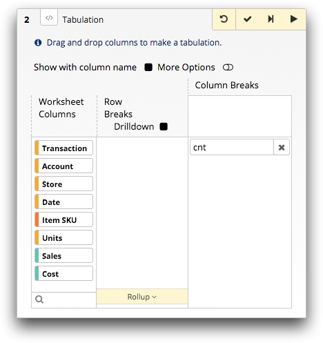 Note: By default, when opened from the New operation panel, the Tabulation panel contains the cnt (count) tabulation function. Otherwise, the New operation panel contains just the column of the selected cell in the Row Breaks section.
 -
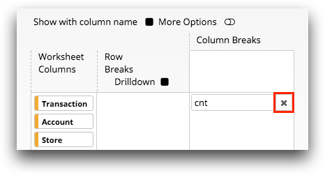
If applicable, remove the default tabulation function by clicking the
Delete Function (
 ) icon in
the field.
) icon in
the field.
-
For each column by which you want to group the records, complete the
following:
-
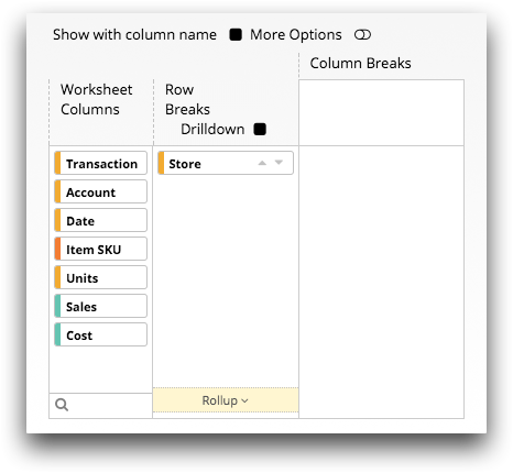
Drag the column from the Worksheet Columns
section to the Row Breaks section.
This selection groups the data by creating a separate row in the resultant worksheet for each unique value within the chosen column. Grouping is a way of pooling all the records for a single entity or value into a single entry in the worksheet.Note: In most cases, the order by which you choose to group the data is important because it can affect the results of the tabulation.The Trillion-Row Spreadsheet moves the column to the Row Breaks section.
-
Optionally, set the sort order of the column by either clicking the
Sort Up (
 ) or
Sort Down (
) or
Sort Down ( )
icon.
)
icon.
All rows that have the same values for all of the columns specified will be considered part of one group.
-
Drag the column from the Worksheet Columns
section to the Row Breaks section.
-
Optional: For each column of data that you want to summarize, complete the
following:
-
Drag the column from the Worksheet Columns
section to the lower area of the Column Breaks
section.
This selection chooses the column of data you want to summarize.
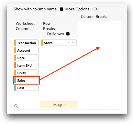 The Trillion-Row Spreadsheet adds a tabulation function field and returns the column to the Worksheet Columns section.Note: By default, columns placed in the lower area of the Column Breaks section are assigned the sum of [COLUMN] summarization. If the data type of the column is text, it is assigned the last of [COLUMN] summarization.
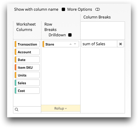
Note: You are not required to provide a tabulation function for a tabulation. You can simply create a list of unique values. -
Drag the column from the Worksheet Columns
section to the lower area of the Column Breaks
section.
-
Optionally, use a rollup in your tabulation.
A rollup provides a subtotal of the summarizations as a row in the resultant worksheet. For instructions, see Use a rollup in a tabulation.
-
Optionally, create a drilldown analysis from the tabulation results.
A drilldown analysis provides an interactive way to explore data points and view row-level data in the grid without changing your underlying query. For instructions, see Set up a drilldown hierarchy.
t0, t1, t2, and so on. You
can give the resultant columns more meaningful names within the More
Options view of the Tabulation panel. In
addition, you can define the various formats of the tabulation
results.-
Optionally, define the format of the tabulation results.
For instructions, see Format the tabulation results.
-
Click the Submit operation (
 ) icon.
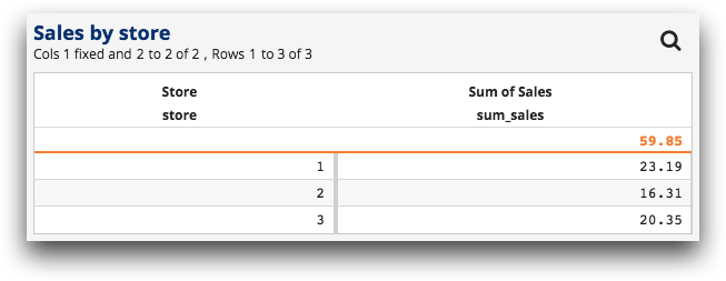
The Trillion-Row Spreadsheet displays the results of your tabulation. You can sort the column breaks like you would any other column.
) icon.
The Trillion-Row Spreadsheet displays the results of your tabulation. You can sort the column breaks like you would any other column.